반응형
In [1]:
import numpy as np
import matplotlib.pylab as plt
퍼셉트론 복습
- 퍼셉트론의 한계
- 사람이 직접 가중치를 찾아야 함
- 신경망
- 사람이 아닌 컴퓨터가 가중치를 찾아낼 수 있음
- 컴퓨터는 주어진 데이터로부터 학습하여 가중치 값을 찾아냄
활성화 함수 1: 계단 함수
In [2]:
# 활성화 함수 1: 계단 함수
def step_function_3(x):
    return np.array(x>0, dtype=np.int) #
x = np.arange(-5.0, 5.0, 0.1)
y = step_function_3(x)
print("y>", y)
print()
print("step function")
plt.plot(x, y)
plt.ylim(-0.1, 1.1)
plt.show()

- 0을 넘지 않는 모든 값들은 0, 0을 넘는 모든 값들은 1
- 이산적(discrete)
활성화 함수 2: 시그모이드(Sigmoid) 함수
In [3]:
# 활성화 함수 2: 시그모이드(Sigmoid) 함수
def sigmoid(x):
    return 1/(1+np.exp(-x)) #

x = np.arange(-5.0, 5.0, 0.1)
y = sigmoid(x)
print("y>", y)
print()
print("sigmoid function")
plt.plot(x, y)
plt.ylim(-0.1, 1.1)
plt.show()

- 0과 1 사이의 값을 가짐
- 극단의 값으로 갈수록 값의 편차가 크지 않음
- 매우 큰 값은 1로 수렴하고 매우 작은 값은 0으로 수렴
- 연속적(continuous)
활성화 함수 3: ReLU(Rectified Linear Unit) 함수
In [4]:
# 활성화 함수 3: ReLU(Rectified Linear Unit) 함수
def relu(x):
    return np.maximum(0, x) #

x = np.arange(-5.0, 5.0, 0.1)
y = relu(x)
print("y>", y)
print()
print("ReLU function")
plt.plot(x, y)
plt.ylim(-0.1, 1.1)
plt.show()

- 0이 넘는 값은 그 입력 그대로 출력, 0을 넘지 못하는 값은 0을 출력
- 다시 말해 모든 양수 값은 그냥 통과, 모든 음수 값은 0으로
- Rectified: 정류된
- 정류 <-> 교류
- 한 방향으로만 흐르는 전류를 만듦
- 0 이하의 입력을 차단하여 아무 값도 출력하지 않게 함
활성화 함수 4: 소프트맥스(Softmax) 함수
In [5]:
# 활성화 함수 5: 소프트맥스(Softmax) 함수
def softmax(x):
    #return (x)/np.sum(np.exp(x))

    e_x = np.exp(x - np.max(x))
    # 지수값의 기하급수적인 증가로 인한 오버플로우 문제(컴퓨터가 표현할 수 있는 값의 범위의 한계를 넘는 것)를 막기 위해서
    # 입력값 각각을 가장 큰 값으로 빼어 스케일링 해준다.
    return e_x / e_x.sum()

x = np.arange(0.0, 3.0, 1)
y = softmax(x)
print("y>", y)
print()
print("softmax function")
# plt.plot(x, y)
# plt.ylim(-0.1, 1.1)
plt.pie(y, labels=y, shadow=True, startangle=90)
plt.show()

- 활성화 함수
- 계단 함수
- 퍼셉트론에서 주로 쓰임
- 계단형
- 시그모이드(Sigmoid) 함수
- 딥 뉴럴 네트워크의 hidden layer에서 주로 쓰임
- s자 형
- p. 68
- ReLU(Rectified Linear Unit) 함수
- 딥 뉴럴 네트워크의 hidden layer에서 주로 쓰이고, 가장 많이 쓰임
- p.76
- 소프트맥스(Softmax) 함수
- 다중분류에서 쓰이며, 출력계층 직전에 쓰임.
- 소프트맥스 함수 출력의 총합은 항상 1 --> 확률로 해석 가능
- p.91
- 계단 함수
- 출력층의 활성화 함수는 풀고자 하는 문제의 성질에 맞게 정한다.
- 예를 들면, 이진분류 문제에는 시그모이드 함수를 쓰고, 다중분류 문제에는 소프트맥스 함수를 사용하는 식이다.
- 모두 비선형함수다.
  - why? p.75 참고
numpy
행렬 생성
In [6]:
A = np.array([1,2,3,4])
print("A")
print(A)
# 배열 A의 차원
print("np.ndim(A): ", np.ndim(A)) #
# A의 shape
print("A.shape: ", A.shape) #
print()
print()
# 2차원 배열 B 생성
B = np.array([[1,2], [3,4], [5,6]]) #
print("B> ")
print(B)
# B의 차원
print("np.ndim(B): ", np.ndim(B))
# (3, 2) B의 shape
print("B.shape: ", B.shape)
In [7]:
# (2, 2) 행렬 A 생성
A = np.array([[1,2], [3,4]]) #
print(A)
print("A.shape: ", A.shape)
print()

# (2, 2) 행렬 B 생성
B = np.array([[5,6],[7,8]]) #
print(B)
print("B.shape: ", B.shape)
print()

# 내적
print("np.dot(A, B)> ") #
print(np.dot(A, B))
행렬의 내적
In [8]:
# (2, 3) 행렬 A 생성
A = np.array([[1,2,3], [4,5,6]]) #
print("A>")
print(A) #
print("A.shape: ", A.shape)
print()

# (3, 2) 행렬 B 생성
B = np.array([[1,2], [3,4], [5,6]]) #
print("B>")
print(B) #
print("B.shape: ", B.shape)
print()

# 내적
print("np.dot(A, B)> ")
print(np.dot(A, B)) #
print()
print("-------------")
print("A>")
print(A) #
print("A.shape: ", A.shape)
print()

# (2, 2) 행렬 C 생성
C = np.array([[1,2],[3,4]]) #
print(C)
print("C.shape: ", C.shape)

# 행렬 A와 행렬 C 내적
np.dot(A, C) #
- 내적에서 한 가지 더 주의할 점은
np.dot(A, B)와np.dot(B, A)가 같지 않다는 점이다.
신경망
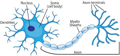
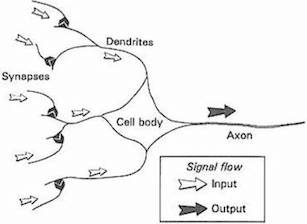
- 생물학에서, 뉴런은 전기적인 신호를 전달받고 전달하는 세포다.
- 신호가 전달되려면 일정 기준(임계값, threshold) 이상의 전기 신호가 존재해야 한다.
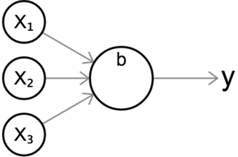
간단한 신경망 구현
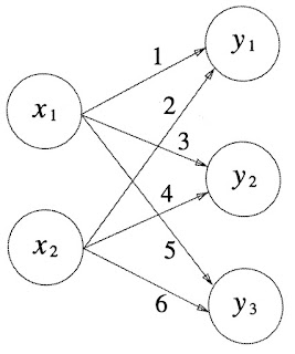
- 내적 연산을 통해서 간단한 신경망 구축 가능
- 신경망은 인간의 입력을
X로, 입력에 대한 가중치를W로,X와W의 곱의 합(곧 내적을 의미함)의 결과를Y로 나타낸다. - 뉴런 여러 개가 모여 층 한 개를 이루고, 층 여러 개가 겹겹이 쌓여 네트워크를 이룬다.
- 층을 여러 개로 쌓을수록 풀려는 문제(또는 대상)에 대한 추상화(또는 모델링, 표현)수준이 높아진다고 함
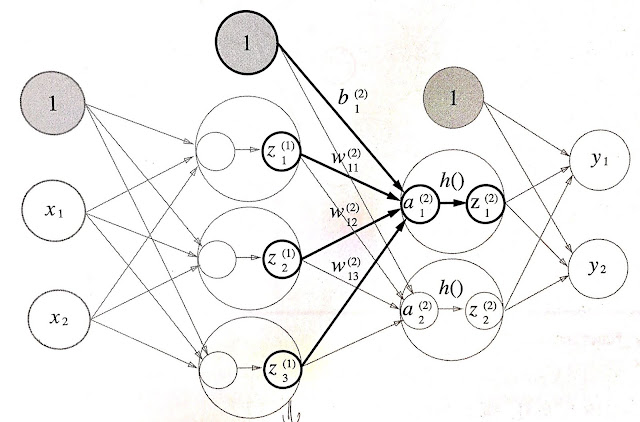
- 신경망의 수학적 모델>
A = XW + BX: 입력, feature(주어짐. 인간이 모델에 제시하는 값.)- 월급, 나이, 성별, 거주지역
W: 가중치(Weight). 구해야 하는 값
어떤 feature에 더 큰 가중치를 둘 것인지 사람이 아닌 신경망이 계산을 통해 Weight들을 찾아낸다. 이에 따라 가중치 값에 따라 feature별로 영향력이 달라진다.B: 편향, 편견(Bias). A값에 영향을 준다. 즉 값이 쉽게 바뀌느냐 마느냐를 결정한다.A: 가중치를 곱한 것들의 합(뉴런의 활성화를 결정하는 값)- "대출 가능/불가능"
- 더 일반적인 표현>
f(X) = b + sum(Wi*Xi)
- 신경망 계산을 사람이 직접 일일이 하지 않고, numpy를 이용하여 행렬의 내적 계산으로 한 번에 계산 가능하다는 장점이 있다.
In [9]:
# 입력이 (2,)인 행렬 X 생성
X = np.array([1,2]) #
X
print("X> ", X)
print()
# 가중치가 (2, 3)인 행렬 W 생성
W = np.array([[1,3,5],[2,4,6]]) #
print("W> ")
print(W)
print()
# X와 W의 내적(요소 별 곱의 합)
Y = np.dot(X, W) #
print("Y> ", Y)
3층 신경망 구현
In [10]:
# 입력층에서 첫번째 Hidden Layer로 전달되는 가중치의 합(A2)과 활성화 함수를 거친 값(Z2)
'''
shape이 (2,)
shape이 (2, 3)
shpae이 (3,)인 행렬 X, W1, B1 생성
'''
X = np.array([1.0, 0.5]) #
W1 = np.array([[0.1, 0.3, 0.5], [0.2, 0.4, 0.6]]) #
B1 = np.array([0.1, 0.2, 0.3]) #

print("X.shape: ", X.shape)
print("W1.shape: ", W1.shape)
print("B1.shape: ", B1.shape)

# 가중치 합
A1 = np.dot(X, W1) + B1
# A1의 값
print("A1> ", A1) #
# 가중치 합에 대한 활성화 함수 적용(시그모이드 함수 적용)
Z1 = sigmoid(A1)
print("Z1> ", Z1)
In [11]:
# 첫번째 Hidden Layer에서 두번째 Hidden Layer로 전달되는 가중치의 합(A2)과 활성화 함수를 거친 값(Z2)
W2 = np.array([[0.1, 0.4], [0.2, 0.5], [0.3, 0.6]])
B2 = np.array([0.1, 0.2])
print("Z1> ", Z1)
print("Z1.shape: ", Z1.shape)
print()
print("W2> ", W2)
print("W2.shape: ", W2.shape)
print()
print("B2> ", B2)
print("B2.shape: ", B2.shape)
A2 = np.dot(Z1, W2) + B2 #
Z2 = sigmoid(A2) #
print()
print("A2> ", A2)
print("A2.shape: ", A2.shape)
print()
print("Z2> ", Z2)
print("Z2.shape: ", Z2.shape)
In [12]:
# 두번째 Hidden Layer에서 출력층으로 전달되는 가중치의 합(A2)과 활성화 함수를 거친 값(Z2)
def identify_function(x):
    return x #
# 활성화 함수 적용이라는 문맥상 흐름에 맞추기 위해

W3 = np.array([[0.1, 0.3], [0.2, 0.4]])
B3 = np.array([0.1, 0.2])
print("Z2> ", Z2)
print("Z2.shape: ", Z2.shape)
print()
print("W3> ", W3)
print("W3.shape: ", W3.shape)
print()
print("B3> ", B3)
print("B3.shape: ", B3.shape)
A3 = np.dot(Z2, W3) + B3 #
Y = identify_function(A3) #
print()
print("A3> ", A3)
print("A3.shape: ", A3.shape)
print()
print("Y> ", Y)
print("Y.shape: ", Y.shape)
In [13]:
def init_network():
    network = {}
    network['W1'] = np.array([[0.1, 0.3, 0.5], [0.2, 0.4, 0.6]])
    network['W2'] = np.array([[0.1, 0.4], [0.2, 0.5], [0.3, 0.6]])
    network['W3'] = np.array([[0.1, 0.3], [0.2, 0.4]])
    network['b1'] = np.array([0.1, 0.2, 0.3])
    network['b2'] = np.array([0.1, 0.2])
    network['b3'] = np.array([0.1, 0.2])

    return network

def forward(network, x): # 왼쪽->오른쪽으로 전개되는 상황을 순전파라고 한다. 역전파도 있으며, 다음 기회에 설명.
    W1, W2, W3 = network['W1'], network['W2'], network['W3']
    b1, b2, b3 = network['b1'], network['b2'], network['b3']

    a1 = np.dot(x, W1) + b1
    z1 = sigmoid(a1)

    a2 = np.dot(z1, W2) + b2
    z2 = sigmoid(a2)

    a3 = np.dot(z2, W3) + b3
    y = identify_function(a3)

    return y

network = init_network()
x = np.array([1.0, 0.5])
y = forward(network, x)
print(y)
- 위 문제의 경우, 3개의 입력을 받아서 2개의 출력을 내는 이진 분류 문제라고 할 수 있음
- 대출 가능,불가 등의 yes, no 문제
In [14]:
# HW
# 1) 아래 코드를 본 후, 다음주까지 네트워크를 손으로 그려오기
#    입력, 가중치, bias, 출력, 활성화 함수가 모두 표현되어 있어야 함

def init_network():
    network = {}
    network['W1'] = np.array([[0.1, 0.3, 0.5, 0.2, 0.4, 0.6, 0.3, 0.6],
                              [0.2, 0.4, 0.6, 0.1, 0.3, 0.5, 0.2, 0.4],
                              [-0.24, 0.46, 0.76, -0.31, 0.33, 0.54, 0.52, 0.44],
                              [0.32, -0.44, 0.86, 0.16, -0.33, -0.51, 0.72, 0.84],
                              [0.72, 0.43, -0.62, 0.18, 0.32, -0.52, 0.12, -0.41]])
    network['W2'] = np.array([[0.1, 0.4, 0.2, 0.5, 0.3, 0.6, 0.3],
                             [0.4, 0.2, 0.1, 0.5, 0.3, 0.6, 0.3],
                             [0.2, 0.5, 0.4, 0.5, 0.1, 0.1, 0.3],
                             [0.5, 0.3, 0.2, 0.5, 0.4, 0.4, 0.1],
                             [0.3, 0.6, 0.5, 0.5, 0.2, 0.2, 0.4],
                             [0.6, 0.3, 0.3, 0.5, 0.5, 0.5, 0.2],
                             [0.3, 0.4, 0.6, 0.5, 0.3, 0.3, 0.5],
                             [0.1, 0.4, 0.3, 0.5, 0.3, 0.6, 0.3]])
    network['W3'] = np.array([[0.1, 0.3, 0.2, 0.4, 0.1],
                             [0.3, 0.3, 0.3, 0.4, 0.9],
                             [0.2, 0.3, 0.2, 0.4, 0.3],
                             [0.4, 0.2, 0.2, 0.4, 0.2],
                             [0.1, 0.4, 0.4, 0.3, 0.4],
                             [0.9, 0.1, 0.2, 0.2, 0.9],
                             [0.1, 0.3, 0.2, 0.4, 0.3]])
    network['W4'] = np.array([[0.1, 0.3, 0.2, 0.4],
                             [0.3, 0.3, 0.3, 0.4],
                             [0.2, 0.3, 0.2, 0.4],
                             [0.4, 0.2, 0.2, 0.4],
                             [0.1, 0.4, 0.4, 0.3]])
    network['W5'] = np.array([[0.1, 0.3, 0.5, 0.2],
                             [0.46, 0.76, -0.31, 0.33],
                             [0.2, -0.62, 0.18, 0.32],
                             [0.4, 0.43, -0.62, 0.4]])
    network['W6'] = np.array([[0.1, 0.3],
                             [0.76, -0.31],
                             [0.18, 0.32],
                             [-0.62, 0.4]])

    network['b1'] = np.array([0.1, 0.2, 0.3, 0.3, -0.3, 0.3, 0.2, 0.2])
    network['b2'] = np.array([0.1, 0.2, 0.3, 0.3, 0.3, 0.3, 0.1])
    network['b3'] = np.array([0.1, 0.1, 0.2, 0.2, 0.3])
    network['b4'] = np.array([0.1, 0.1, 0.2, 0.2])
    network['b5'] = np.array([0.1, 0.1, 0.2, 0.2])
    network['b6'] = np.array([0.1, 0.1])

    return network

def forward(network, x):
    W1, W2, W3, W4, W5, W6 = network['W1'], network['W2'], network['W3'], network['W4'], network['W5'], network['W6']
    b1, b2, b3, b4, b5, b6 = network['b1'], network['b2'], network['b3'], network['b4'], network['b5'], network['b6']

    a1 = np.dot(x, W1) + b1
    z1 = sigmoid(a1)

    a2 = np.dot(z1, W2) + b2
    z2 = sigmoid(a2)

    a3 = np.dot(z2, W3) + b3
    z3 = sigmoid(a3)

    a4 = np.dot(z3, W4) + b4
    z4 = relu(a4)

    a5 = np.dot(z4, W5) + b5
    z5 = relu(a5)

    a6 = np.dot(z5, W6) + b6
    y_softmax = softmax(a6)
    y_identify_function = identify_function(a6)

    return y_softmax, y_identify_function

network = init_network()
x = np.array([1.0, 0.5, 0.4, 0.9, -1.3])
y_softmax, y_identify_function  = forward(network, x)
print("{:25s}: {}".format("y_identify_function: ", y_identify_function))
print("{:25s}: {}".format("y_softmax: ", y_softmax))
Neural Network가 할 일은, 1)가장 적합한 파라미터를 찾아내어, 2)결과값을 개선하는 것이다.
- 즉 훈련 데이터(학습 데이터)를 사용하여 가중치 매개변수를 학습한 후, --> 학습 단계 : 다음 시간(역전파 파트 때)에.
- 학습하여 구한 매개변수를 이용하여 새로운 입력 데이터를 예측 또는 분류해낸다. --> 추론 단계
- 출력층의 뉴런수는 풀려는 문제에 맞게 적절히 정해야 한다.
- 분류문제의 경우, 분류하려는 클래스의 개수에 맞게 출력층의 뉴런 개수를 정하는 것이 일반적
- Yes, no -> 출력층에 두 개의 뉴런
- MNIST -> 0~9까지 10개의 뉴런
MNIST
- 손글씨 숫자 이미지 집합
기계학습의 대표적인 데이터셋, 성능 벤치마크 기준
- 데이터 집합
- 연령, 나이, 연봉, 직업, 사는지역, [대출상환여부:1/0]
- 매개변수 학습에 쓰이는 데이터셋을 훈련 데이터셋(training dataset)
- 모델의 성능을 측정하고, 좋은 모델을 선택하기 위해 쓰이는 검증 데이터셋(validation dataset). 모델의 학습시에는 쓰일 때도 있고 쓰이지 않을때도 있다.
- 최종적인 모델이 얼마나 좋은지를 평가하기 위해 쓰이는 시험 데이터셋(test dataset). 학습시에는 절대 쓰이지 않는다.
MNIST는 0부터 9까지의 손글씨 숫자를 이미지화 한 데이터셋
- 훈련 이미지: 60,000장
- 시험 이미지: 10,000장
http://yann.lecun.com/exdb/mnist/


- 784(=28*28) 사이즈의 그레이 스케일 이미지 -->
1x28x28 - 각각의 필셀값은 0부터 255(2^8)까지의 값을 갖음
- MNIST 데모: https://ml4a.github.io/demos/forward_pass_mnist/
MNIST 데이터셋 -> numpy.ndarray
In [15]:
# coding: utf-8
try:
    import urllib.request
except ImportError:
    raise ImportError('You should use Python 3.x')
import os.path
import gzip
import pickle
import os
import numpy as np


url_base = 'http://yann.lecun.com/exdb/mnist/'
key_file = {
    'train_img':'train-images-idx3-ubyte.gz',
    'train_label':'train-labels-idx1-ubyte.gz',
    'test_img':'t10k-images-idx3-ubyte.gz',
    'test_label':'t10k-labels-idx1-ubyte.gz'
}

dataset_dir = os.getcwd() #os.path.dirname(os.path.abspath(__file__))
save_file = dataset_dir + "/mnist.pkl"

train_num = 60000
test_num = 10000
img_dim = (1, 28, 28)
img_size = 784


def _download(file_name):
    file_path = dataset_dir + "/" + file_name

    if os.path.exists(file_path):
        return

    print("Downloading " + file_name + " ... ")
    urllib.request.urlretrieve(url_base + file_name, file_path)
    print("Done")

def download_mnist():
    for v in key_file.values():
        _download(v)

def _load_label(file_name):
    file_path = dataset_dir + "/" + file_name

    print("Converting " + file_name + " to NumPy Array ...")
    with gzip.open(file_path, 'rb') as f:
            labels = np.frombuffer(f.read(), np.uint8, offset=8)
    print("Done")

    return labels

def _load_img(file_name):
    file_path = dataset_dir + "/" + file_name

    print("Converting " + file_name + " to NumPy Array ...")
    with gzip.open(file_path, 'rb') as f:
            data = np.frombuffer(f.read(), np.uint8, offset=16)
    data = data.reshape(-1, img_size)
    print("Done")

    return data

def _convert_numpy():
    dataset = {}
    dataset['train_img'] =  _load_img(key_file['train_img'])
    dataset['train_label'] = _load_label(key_file['train_label'])
    dataset['test_img'] = _load_img(key_file['test_img'])
    dataset['test_label'] = _load_label(key_file['test_label'])

    return dataset

def init_mnist():
    download_mnist()
    dataset = _convert_numpy()
    print("Creating pickle file ...")
    with open(save_file, 'wb') as f:
        pickle.dump(dataset, f, -1)
    print("Done!")

def _change_one_hot_label(X):
    T = np.zeros((X.size, 10))
    for idx, row in enumerate(T):
        row[X[idx]] = 1

    return T


def load_mnist(normalize=True, flatten=True, one_hot_label=False):
    """MNIST 데이터셋 읽기

    Parameters
    ----------
    normalize : 이미지의 픽셀 값을 0.0~1.0 사이의 값으로 정규화할지 정한다.
    one_hot_label :
        one_hot_label이 True면、레이블을 원-핫(one-hot) 배열로 돌려준다.
        one-hot 배열은 예를 들어 [0,0,1,0,0,0,0,0,0,0]처럼 한 원소만 1인 배열이다.
    flatten : 입력 이미지를 1차원 배열로 만들지를 정한다. 본래는 1*28*28의 3차원 이미지.

    Returns
    -------
    (훈련 이미지, 훈련 레이블), (시험 이미지, 시험 레이블)
    """
    if not os.path.exists(save_file):
        init_mnist()

    with open(save_file, 'rb') as f:
        dataset = pickle.load(f)

    if normalize:
        for key in ('train_img', 'test_img'):
            dataset[key] = dataset[key].astype(np.float32)
            dataset[key] /= 255.0

    if one_hot_label:
        dataset['train_label'] = _change_one_hot_label(dataset['train_label'])
        dataset['test_label'] = _change_one_hot_label(dataset['test_label'])

    if not flatten:
         for key in ('train_img', 'test_img'):
            dataset[key] = dataset[key].reshape(-1, 1, 28, 28)

    return (dataset['train_img'], dataset['train_label']), (dataset['test_img'], dataset['test_label'])


if __name__ == '__main__':
    init_mnist()
훈련 데이터, 시험 데이터
In [16]:
(x_train, t_train), (x_test, t_test) = load_mnist(flatten=True, normalize=False, one_hot_label=False)
# (x_train, t_train), (x_test, t_test) = load_mnist(flatten=True, normalize=True, one_hot_label=False)
# (x_train, t_train), (x_test, t_test) = load_mnist(flatten=True, normalize=True, one_hot_label=True)
print("x_train> ")
print(x_train)
print("x_train.shape: ", x_train.shape)
print("x_train[0][230:250]> ", x_train[0][230:250])
print("x_train[0].shape> ", x_train[0].shape)
print()
print("t_train> ")
print(t_train)
print("t_train.shape: ", t_train.shape)
print("t_train[0]> ", t_train[0])
print("t_train[0].shape> ", t_train[0].shape)
print()
print("x_test> ")
print(x_test)
print("x_test.shape: ", x_test.shape)
print("x_test[0][230:250]> ", x_test[0][230:250])
print("x_test[0].shape> ", x_test[0].shape)
print()
print("t_test> ")
print(t_test)
print("t_test.shape: ", t_test.shape)
print("t_test[0]> ", t_test[0])
print("t_test[0].shape> ", t_test[0].shape)
print()
MNIST 숫자 분류/추론
In [37]:
def get_data():
    (x_train, t_train), (x_test, t_test) = load_mnist(normalize=True, flatten=True, one_hot_label=False)
    return x_test, t_test


def init_network():
    with open("sample_weight.pkl", 'rb') as f:
        network = pickle.load(f)
    return network


def predict(network, x):
    W1, W2, W3 = network['W1'], network['W2'], network['W3']
    b1, b2, b3 = network['b1'], network['b2'], network['b3']

    a1 = np.dot(x, W1) + b1
    z1 = sigmoid(a1)
    a2 = np.dot(z1, W2) + b2
    z2 = sigmoid(a2)
    a3 = np.dot(z2, W3) + b3
    y = softmax(a3)

    return y


x, t = get_data()
network = init_network()
print("x.shape: ", x.shape)
print("x[0].shape: ", x[0].shape)
print("batchsize * x[0].shape: ({}, {})".format(1, x[0].shape[0])) # 개념적인 표현
print("network['W1'].shape: ", network['W1'].shape)
print("network['W2'].shape: ", network['W2'].shape)
print("network['W3'].shape: ", network['W3'].shape)
print("output layer's shape: ({}, {})".format(1, 10)) # 개념적인 표현
print()
accuracy_cnt = 0
for i in range(len(x)): # 불러온 이미지 x를 한 장씩 꺼내서 predict()함수에 넣는다. predict()함수는 이미지가 어떤 숫자인지 분류/추론한다.
    y = predict(network, x[i]) # softmax이므로 0.0과 1.0사이의 확률값으로 나옴
    p= np.argmax(y) # 확률값이 가장 높은 원소의 인덱스를 얻는다.
    if p == t[i]: # 예측한 결과인 p와 실제 정답인 t[i]를 비교
        accuracy_cnt += 1

print("Accuracy:" + str(float(accuracy_cnt) / len(x))) # 93.52%의 정확도로 정확하게 분류
- 세 개의 Layer
- sample_weight.pkl
- 미리 학습된 모델의 매개변수를 불러옴
- 학습 과정은 다음 시간에.
- 입력층의 뉴런수: 784
- 첫번째 은닉층의 뉴런수: 50
- 두번째 은닉층의 뉴런수: 100
- 출력층의 뉴런수: 10
배치 처리
- 이미지를 여러 장을 하나로 묶어서 한꺼번에
predict()에 넣고자 할 때- 하나로 묶은 입력 데이터를 배치(batch)라 함
In [36]:
def get_data():
    (x_train, t_train), (x_test, t_test) = load_mnist(normalize=True, flatten=True, one_hot_label=False)
    return x_test, t_test


def init_network():
    with open("sample_weight.pkl", 'rb') as f:
        network = pickle.load(f)
    return network


def predict(network, x):
    w1, w2, w3 = network['W1'], network['W2'], network['W3']
    b1, b2, b3 = network['b1'], network['b2'], network['b3']

    a1 = np.dot(x, w1) + b1
    z1 = sigmoid(a1)
    a2 = np.dot(z1, w2) + b2
    z2 = sigmoid(a2)
    a3 = np.dot(z2, w3) + b3
    y = softmax(a3)

    return y

accuracy_cnt = 0

x, t = get_data()
network = init_network()
batch_size = 100 # 배치 크기

# for i in range(len(x)):
#     y = predict(network, x[i])
#     p= np.argmax(y)
#     if p == t[i]:
#         accuracy_cnt += 1

for i in range(0, len(x), batch_size):
    y_batch = predict(network, x[i:i+batch_size])
    p = np.argmax(y_batch, axis=1)
    accuracy_cnt += np.sum(p == t[i:i+batch_size])

print("x.shape: ", x.shape)
print("x[0].shape: ", x[0].shape)
print("batchsize * x[0].shape: ({}, {})".format(batch_size, x[0].shape[0])) # 개념적인 표현
print("network['W1'].shape: ", network['W1'].shape)
print("network['W2'].shape: ", network['W2'].shape)
print("network['W3'].shape: ", network['W3'].shape)
print("output layer's shape: ({}, {})".format(batch_size, 10)) # 개념적인 표현
print()
print("Accuracy:" + str(float(accuracy_cnt) / len(x)))
- 배치 처리의 이점
- 계산 효율: 큰 배열을 효율적으로 처리할 수 있도록 최적화되어 있음
- I/O 횟수를 줄여 버스 부하를 줄임 --> 계산 속도 향상에 도움을 줌
반응형
'Artificial Intelligence > Deep Learning' 카테고리의 다른 글
| 정규화 (0) | 2018.12.23 |
|---|---|
| Batch 크기의 결정 방법 (0) | 2018.12.23 |
| coursera_week2_6_Derivatives with a Computation Graph (1) | 2017.10.04 |
| coursera_week2_5_Computation Graph (0) | 2017.10.04 |
| coursera_week2_4_Gradient Descent (0) | 2017.10.04 |